


This blog helps you to understand how to build an end-to-end Face Expression Detection using Keras and CNN's.
1. Problem
Identifying the face expression of a human, given an image of him/her.
2. Data
Data is taken from Kaggle's Facial Expression Recognition Challenge: kaggle.com/c/challenges-in-representation-l..
Currently the data from above official Kaggle link is not available. So we can take the same data from : kaggle.com/shawon10/facial-expression-detec..
3. Evaluation
Evaluation is done based on accuracy and loss between predicted expression and actual expression.
4. Features
Some information about the data:
- We're dealing with images(unstructured data), so better we use deep learning / transfer learning.
- Data has 3 columns namely emotions, picture, and usage(Training/Testing).
- Data has 35887 rows(images).
- There are 28709 training images (with column value as Training).
- There are 3589 testing images (with column value as PublicTest).
- PrivateTest records are ignored as of now.
- Data has 7 classes (emotions).
- 0=Angry
- 1=Disgust
- 2=Fear
- 3=Happy
- 4=Sad
- 5=Surprise
- 6=Neutral
Note: I would be discussing the implementation process and code snippets here. However, if you want to replicate the same results, please feel free to use my entire code which is provided as a link at the end of this article.
Getting our workspace ready
I have opted to work on google colab since it offers a free GPU. However we can run the enitre code(which we will be discussing) even on your personal computer.
Import all the standard libraries which we will be using and define the define the base_path parameter.
import tensorflow as tf
import keras
import numpy as np
import pandas as pd
import matplotlib.pyplot as plt
import cv2

base_path = "drive/My Drive/Expression Detection/"
%matplotlib inline
Check GPU availability
# Check for GPU availability
print("GPU ", "available :) !!" if tf.config.list_physical_devices("GPU") else "not available :(")
Note: We can run the model even without GPU, but it would take a bit more for model training.
Getting our data ready
Download the fer2013.csv.zip file from the above mentioned Kaggle link and upload it to the project folder in google colab. Unzip the uploaded dataset.
!unzip "drive/My Drive/Expression Detection/fer2013.csv.zip" -d "drive/My Drive/Expression Detection/"
Exploring the data
It is always a good practice to do some EDA(Exploratory Data Analysis) on our data before starting to use it. This helps us to know more about data.
We can do things like:
Load the entire data into a pandas DataFrame
raw_dfChecking for number of columns
raw_df.columnsChecking for total number of records and their data_types
raw_df.info()Checking for total number of unique classes
raw_df["emotion"].value_counts()Checking for total number of training and testing images
raw_df[raw_df['Usage'] == "Training"], raw_df[raw_df["Usage"] == "PrivateTest"]Checking for distribution of various emotions(classes) in the dataset.
# Check the distribution of various emotions in the dataset
x_labels = ['angry', 'disgust', 'fear', 'happy', 'sad', 'surprise', 'neutral']
plt.figure(figsize=(10,5))
ax = raw_df["emotion"].value_counts().plot(kind='bar')
ax.set_xticklabels(x_labels);
ax.tick_params(axis='x', colors='lightblue', rotation=45)
ax.tick_params(axis='y', colors='lightblue')
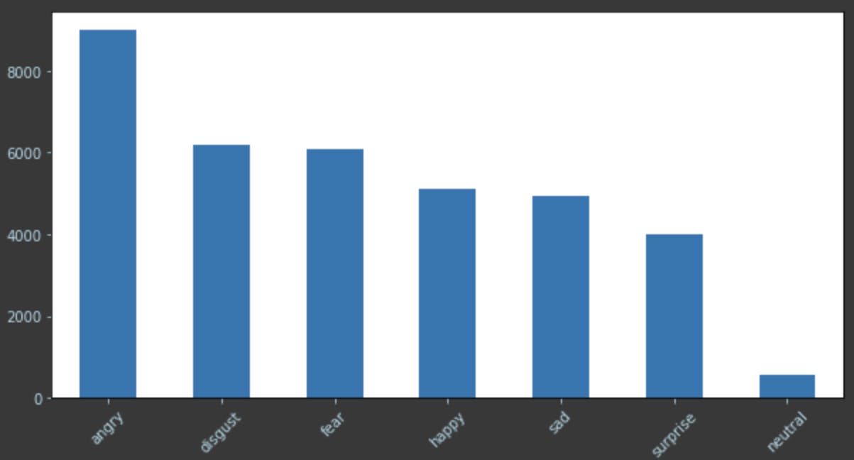
From the previous check we can understand that, classes are not distributed uniformly. Angry, Neutral classes are outliers, this may lead to making to our model do wrong predictions. To avoid this we can do some data augmentation and make the classes distribution uniform. However, for sake of simplicity we will proceed with current dataset.
Creating Training and Test datasets
Our dataset is classified into 3 parts : Training, PublicTest, PrivateTest. Consider Training part as our training dataset and PublicTest as our testing dataset. Ignore PrivateTest data for now. Now, we can create our training and testing datasets using the below snippet.
# Loop through the entire dataframe
for index, row in raw_df.iterrows():
  # transform pixels
  pixels_val = row["pixels"]
  pixels = np.array(pixels_val.split(" "), dtype='float32')

  # transform emotions
  emotion_val = row["emotion"]
  emotion = keras.utils.to_categorical(emotion_val, num_classes=num_classes)

  # Split the data based on usage
  usage = row["Usage"]

  if "Training" in usage:
    X_train.append(pixels)
    y_train.append(emotion)
  elif "PublicTest" in usage:
    X_test.append(pixels)
    y_test.append(emotion)
Current training and test data sets are in the form of lists, we need to convert them into numpy arrays for further processing.
X_train = np.array(X_train, dtype='float32')
y_train = np.array(y_train, dtype='float32')
X_test = np.array(X_test, dtype='float32')
y_test = np.array(y_test, dtype='float32')
Since inputs (X_train, X_test) hold the pixel values, they range from 0 to 255. We need to normalize them between 0 to 1.
# Normalize the inputs between [0, 1]
X_train /= 255
X_test /= 255
Next, reshape the data from 1D(28709) to 3D(48,48,1).
# Reshape each value from 1D(28709) to 3D(48,48,1)

X_train = X_train.reshape(X_train.shape[0], 48, 48, 1)
X_train = X_train.astype('float32')
X_test = X_test.reshape(X_test.shape[0], 48, 48, 1)
X_test = X_test.astype('float32')

print(X_train.shape[0], 'train samples')
print(X_test.shape[0], 'test samples')
Batichfy the data
We can load our data to the model either in the form of batches or as a whole set. But, tensorflow(Keras uses tenforflow at backend) works best when data is given in the form of batches. The GPU and tensorflow at backend will try to distribute the training process across all the available cores. Each core will be training the model with a seperate batch of data.
We can turn the data into batches with the below snippet.
from keras.preprocessing import image
from keras.preprocessing.image import ImageDataGenerator

# Turn data to batches
batch_size = 256
gen = ImageDataGenerator()
train_generator = gen.flow(X_train, y_train, batch_size = batch_size)
Construct a CNN (Convolutional Neural Network)
Create a model
Here we can start with Keras-Sequential as our base model.
Initialize a Sequential model.
Add three 2D convolution layers with activation function as
relu.Flatten the output.
Add an output layer with activation function as
softmaxand num_classes as 7( one each for angry, disgust, fear, happy, sad, surprise, neutral). This means that, at starting input layer we will have 2304 neurons which will then be converged to final 7 neurons(angry, disgust, fear, happy, sad, surprise, neutral) with the help of 3 convolutional layes and their respective activation functions.Since it is multi-class classification problem, we will use
categorical_crossentropyas loss function,Adamas optimizer,accuracyas metrics.
This snippet for model creation is as below:
from keras.models import Sequential
from keras.layers import Conv2D, MaxPooling2D, AveragePooling2D
from keras.layers import Dense, Activation, Dropout, Flatten

model = Sequential()

# 1st Convolutionla layer
model.add(Conv2D(64, (5,5), activation='relu', input_shape=(48,48,1)))
model.add(MaxPooling2D(pool_size=(5,5), strides=(2,2)))

# 2nd Convolutionla layer
model.add(Conv2D(64, (3,3), activation='relu'))
model.add(Conv2D(64, (3,3), activation='relu'))
model.add(AveragePooling2D(pool_size=(3,3), strides=(2,2)))

# 3rd Convolutionla layer
model.add(Conv2D(128, (3,3), activation='relu'))
model.add(Conv2D(128, (3,3), activation='relu'))
model.add(AveragePooling2D(pool_size=(3,3), strides=(2,2)))

model.add(Flatten())

# Fully connected Neural Network
model.add(Dense(1024, activation='relu'))
model.add(Dropout(0.2))
model.add(Dense(1024, activation='relu'))
model.add(Dropout(0.2))
model.add(Dense(num_classes, activation='softmax'))

# Compile the model
model.compile(loss='categorical_crossentropy',
              optimizer=keras.optimizers.Adam(),
              metrics=['accuracy'])
Fit the model
The fit method will load the data(in the form of batches) to the model and start training. The epocs here is set to 30. However, for this model with this set of data, ideal epoc value can range between 25 to 30. Upon triaing with 30 epochs, my model has achieved nearly 90% accuracy on the training data.
fit = True

if fit == True:
  # Train the model on the entire data set
  model.fit_generator(train_generator, steps_per_epoch=batch_size, epochs=epochs, verbose=1)

  #Saving the model as a single .hdf5 file
  save_model(model, save_method='Pickle')
else:
  # load weights
  #model.load_weights('drive/My Drive/Expression Detection/facial_expression_model_weights.h5')
  pass
A bit about epoch
Epochs are like how many rounds of training the model has to undergo. First epoch will take more time and subsequent epochs will be faster. This can be better explained with the help of an example:
Think a student is preparing for his exam. He has to study all the chapters so that he can answer the questions in the exam. For the first time, he takes a week to study entire syllabus. But after that, when he revises the syllabus again he can do it in a day since he has done most of the learning during first time. Simlarly, for further revisions he can do even more fastly(may be within hours). The more he revises, the more he is confident to perform well in the exam. Here the model is the student, each revision is an epoch and exam is test predictions.
Saving the model
We can save a model using two methods.
- Using Keras in-built
save()method. - Using Pickle
dump()method.
import pickle

# Save a model using either uisng Keras `save()` method or Picke `dump()` method

def save_model(model, save_method='Keras'):
  if save_method == 'Keras':
    # Method 1: Using Keras. Will be save as a single .hdf5 file
    model.save(base_path+'model30.hdf5')
  elif save_method == 'Pickle':
    # Method 2 : Usign pickle
    with open(base_path+'model30.pkl', 'wb') as file:
      pickle.dump(model, file)

  print("Model saved.")

save_model(model, save_method='Pickle')
Load the saved model
Similar to saving a model, we can load the model in two ways:
- Using Keras
load_model() - Using Pickle
load()The loaded model can be directly used of prediction.
import pickle

# Load a model using Keras or Pickle

def load_model(load_method='Keras'):
  model = None
  if load_method == 'Keras':
    # Method 1: Using Keras
    model = keras.models.load_model(base_path+'model30.hdf5')
  elif load_method == 'Pickle':
    # Method 2: Using Pickle
    with open(base_path+f'model30.pkl', 'rb') as f:
      model = pickle.load(f)

  print("Model Loaded.")
  return model

loaded_model = load_model(load_method='Keras')
Evaluate the trained model
Now as we have fully trained our model, let's make some predictions on the test data and evalute the model.
Use the evaluate() method to evalute the trained model against train and test dataset
train_score = loaded_model.evaluate(X_train, y_train, verbose=1)
print(f"Train loss : {train_score[0]}")
print(f"Train accuracy : {train_score[1]}")
test_score = loaded_model.evaluate(X_test, y_test, verbose=1)
print(f"Test loss : {test_score[0]}")
print(f"Test accuracy : {test_score[1]}")
Confusion Matrix
A Confusion Matrix helps us to analyze where our model is getting confused.
Plotting a confusin matrix between predicted labels and truth(ground) labels
from sklearn.metrics import confusion_matrix
import seaborn as sn

label_names = ['angry', 'disgust', 'fear', 'happy', 'sad', 'surprise', 'neutral']
label_values = [0,1,2,3,4,5,6]

# Make a predictions predictions list
y_preds = loaded_model.predict(X_test)
y_preds_mod, y_test_mod = [], []

for pred in y_preds:
  y_preds_mod.append(np.argmax(pred))

for truth in y_test:
  y_test_mod.append(np.argmax(truth))

# Create a confusion matrix
cm = confusion_matrix(y_test_mod, y_preds_mod, labels=label_values)

# Visualize the confusion matrix using Seaborn heatmap
df_cm = pd.DataFrame(cm,
                     index=label_names,
                     columns=label_names)
plt.figure(figsize=(10,5))
sn.heatmap(df_cm, annot=True, fmt='g');
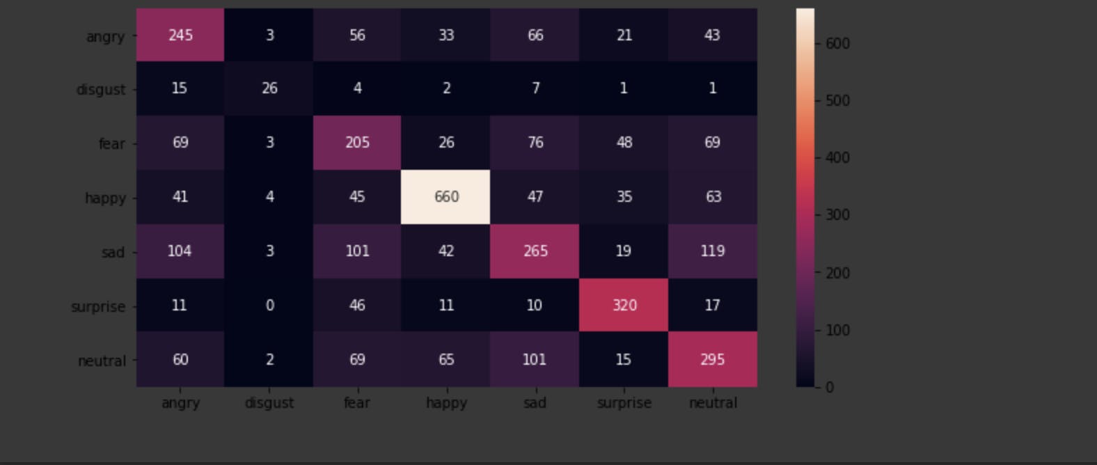
From the confusion matrix, we can derive the following observations:
- Our model is not getting confused for Happy and suprise classes. It has predicted correctly more than 90%. So we can confidently say that our model will do good for Happy & Suprise faces.
- For other labels, the model is pretty much confused. However, we can handle this if we want by various means:
- Making the data uniform for all labels.
- Making the data rich by adding wild images downloaded form internet.
- Add more hidden(convultional) layers to our CNN.
Helper function to visualize the test results
To better understand and visualize the test results, we can create a helper function which will plot the test image and its test predictions.
def def analyze_emotion(emotions):
  label_values = ['angry', 'disgust', 'fear', 'happy', 'sad', 'surprise', 'neutral']
  y_seq = np.arange(len(label_values))

  plt.bar(y_seq, emotions, align='center', alpha=0.5)
  plt.xticks(y_seq, labels=label_values)
  plt.ylabel('Percentage')
  plt.title('Emotion')
  plt.show()(emotions):
  label_values = ['angry', 'disgust', 'fear', 'happy', 'sad', 'surprise', 'neutral']
  y_seq = np.arange(len(label_values))

  plt.bar(y_seq, emotions, align='center', alpha=0.5)
  plt.xticks(y_seq, labels=label_values)
  plt.ylabel('Percentage')
  plt.title('Emotion')
  plt.show()
Testing the model with real-time data
Reduce noise in testing images using openCV2 and Haarcascade model.
Before sending our custom image to the model for prediction, we have to make sure that all the un-necessary part of the image is removed. Haarcascade model with the help of openCV2 automatically detects the face in the model and trims the remaining part. Doing so, will make our model less confused and predict well.
Create a function named face_crop() which will achieve the above behaviour.
def face_crop(image):
  face_data = base_path + 'haarcascade_frontalface_alt.xml'
  cascade = cv2.CascadeClassifier(face_data)
  img = cv2.imread(image)
  if (img is None):
    print("Can't open image file")
    return 0

  try:

    minisize = (img.shape[1], img.shape[0])
    miniframe = cv2.resize(img, minisize)

    faces = cascade.detectMultiScale(miniframe)
    if (faces is None):
      print('Failed to detect face')
      return 0

    facecnt = len(faces)
    print("Detected faces: %d" % facecnt)

    for f in faces:
      x, y, w, h = [v for v in f]
      cv2.rectangle(img, (x,y), (x+w,y+w), (0,255,0), 2)
      sub_face = img[y:y+h, x:x+w]
      cv2.imwrite(base_path+'data/capture.jpg', sub_face)

      #cv2.imwrite(image, sub_face)

    print("crop completed.")

  except Exception as e:
    print(e)
Use the above function to crop the face in our custom image and then send the image to our model for prediction.
Predict custom faces
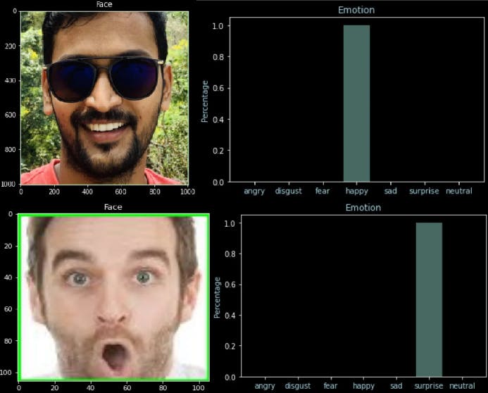
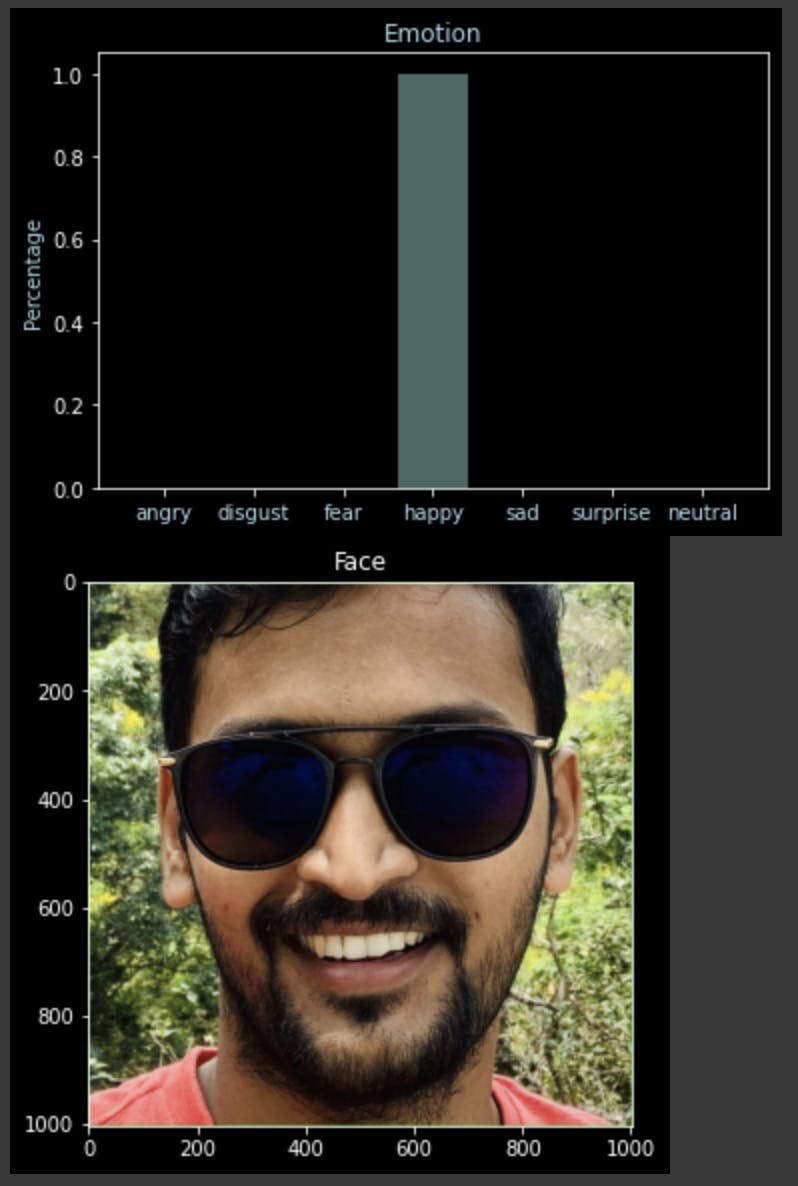
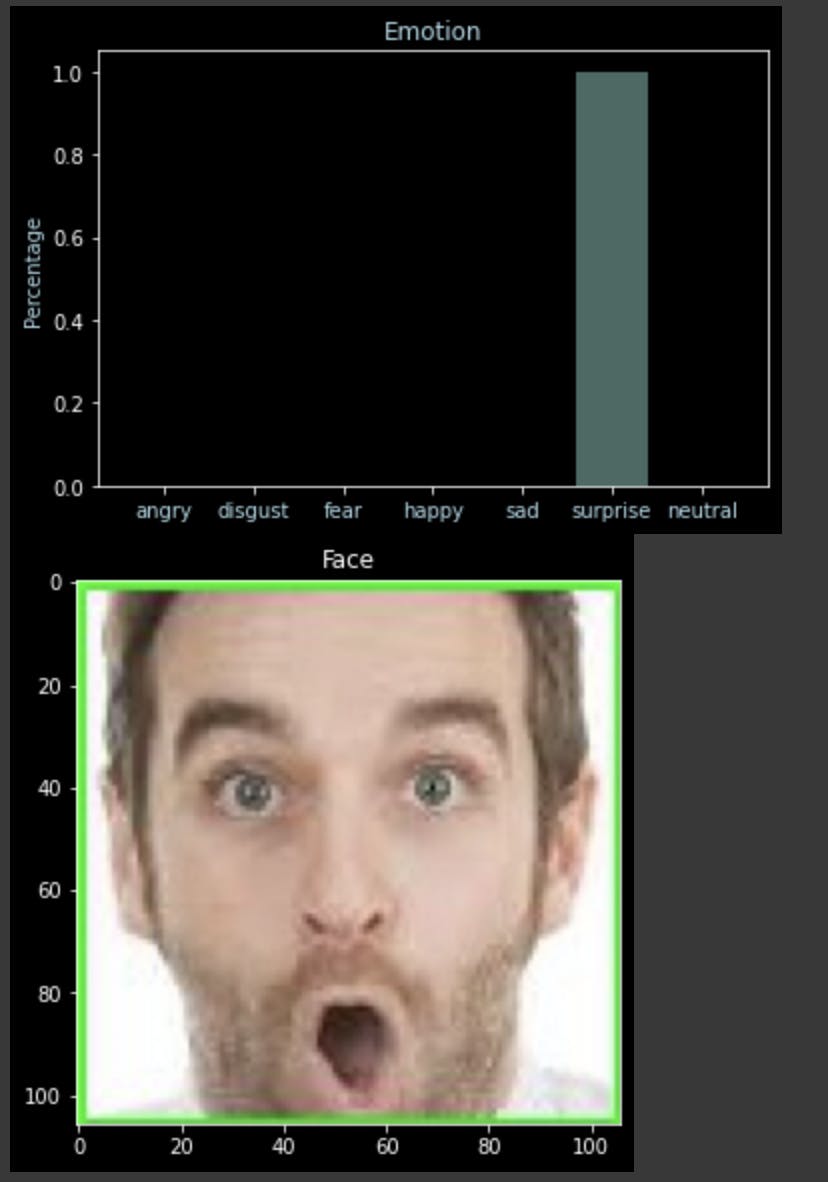
Now, as our model is ready, we will use the pedict() function and our helper function analyze_emotion() to see the predictions.
file = "drive/My Drive/Expression Detection/data/capture.jpg"
actual_image = image.load_img(file)
img = image.load_img(file, color_mode='grayscale', target_size=(48,48))

X_custom = image.img_to_array(img)
X_custom = np.expand_dims(X_custom, axis=0)

#normalize the cusotm input
X_custom /= 255

y_custom = loaded_model.predict(X_custom)
analyze_emotion(y_custom[0])


plt.gray()
plt.imshow(actual_image)
plt.show()
Improvements:
- Enrich the dataset: As discussed above, the target classes(labels) are not distributed uniformly across the given dataset. So, we can use some web scrapping tools which are freely available on intrenet to download bulk images of a specific kind. I have found a cool tool, Google Image Downloads which will do the job.
- Try with different model: Since I have decided to do transfer learning, i haved picked up Keras Sequential model. There are so many other models for image classification and FER(Facial Expression Recognition) available, you can try exploring them aswell.
- Deploy the trained model to web app using Falsk and Heroku.
Full Code:
📚 Please find the full notebook code in my GitHub repository.
💻 Look out to my GitHub Profile for other Data Science and ML projects.
👨💻 My Site : https://bharatkammakatla.com
Conclusion
Finally, by using Transfer Learning, Keras, Convolutional Neural Network's we have created a machine learning model capable of identifying facial expressions.
That's it Guyz ✅ !!
Hope you liked it. If so, hit a like 👍.
For any suggestions or queries, please feel free to comment below ✍️.
Thanks for reading the post. Have nice day 😀.